Modmain is a graphical user interface for MODFLOW, the MODular three- dimensional, finite difference FLOW model developed by the United States Geological Survey (McDonald and Harbaugh, 1984). MODFLOW is a program designed to model ground water flow and heads (pressure and elevation) in confined and unconfined aquifer systems. In its basic form, MODFLOW can be difficult, or awkward to use. The modmain program module is designed to simplify data entry, model editing, and analysis of results.

This chapter goes into the details of using modmain as an interface for MODFLOW. It however does not explain the theory or use of MODFLOW, that is better left to the MODFLOW user's manual (McDonald and Harbaugh, 1984).

WARNING: To use modmain and MODFLOW effectively, you must have the MODFLOW user's manual, and it should be readily available whenever you are building data sets with modmain. In the current release, modmain does not error check data file formats; this can lead to incorrect numbers for any variable, and it can cause "segmentation faults" which will terminate modmain. To find the problem, the data files may have to be examined line by line to determine where the problem is. This can only be done if the MODFLOW user's manual is available!

The modmain application is composed of two sections; the main menu-bar, and the status and log text area. The menu-bar is used to select all modmain commands, and the log/status area is used by the program to report important messages or results. In addition to the main window and supporting pop-up dialog windows, a graphical editor is available for creating and modifying two-dimensional arrays. Modmain also use's other UNCERT (grid, contour, surface, and block) modules for visualizing model output.

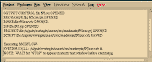Figure 15.1

[TOP] [SYNTAX]

Open Project:

View Project:

Save Project:

Save Preferences:

WARNING: if modmain.prf" already exists, you will be warned that it is about to be over-written. If you do not want the old version destroyed you must move it to a new file (e.g. the UNIX command mv modmain.prf modmain.old.prf would be sufficient). When you press OK the old version will be over-written! This cannot be done currently from within the application. To rename the file, you will have to execute the UNIX mv command from a UNIX prompt in another window.

If "modmain.prf" does not exist in the current directory, it is created. This is an ASCII file and can be edited by the user. See Appendix C for details.

Quit:

Quit Without Saving:

[TOP] [SYNTAX]

NOTE: When first starting modmain, a project must be loaded, a Basic package file must be loaded, or a Basic package must be created (Packages:Basic:Modify menu option) before any package besides the Basic package can be read or created. This is because the Basic package contains the grid row, column, layer dimension information that all of the other packages require.

Each package has a pull-down sub-menu with five menu options: Open Package, View Package:Save, Save as, and Modify. The Open option generates a dialog similar to that shown in Figure 5.2. The dialogs works the same as that dialog too, except that the default file name extensions are different. For each package the default file name extensions are:

BASIC: *.bas
BLOCK CENTERED FLOW: *.bcf
DRAIN: *.drn
EVAPOTRANSPIRATION: *.evt
GENERAL HEAD: *.ghb
OUTPUT CONTROL: *.oc
PCG2: *.pcg
RECHARGE: *.rch
RIVER: *.riv
SIP: *.sip
SSOR: *.ssor
WELL: *.well

These file extensions are strictly conventions, and do not have to be followed. It, however, is recommended that you follow some consistent naming convention. The View menu option will display the last saved or loaded version of the data file.

NOTE: Changes made to a package within the modmain application (using Modify below) will not be reflected in the data file until the changes have been saved (see Save below).

The Save menu option will save any modifications, overwriting the last opened or saved package file. If no package file has been loaded or saved previously, a pop-up dialog will appear similar to Figure 5.2's, but showing the appropriate default file extension. To save the package file, select an existing file, or enter a new file name, then press the "Save" button on the dialog. Save as is similar to Save, except that you are queried for a file name. Modify will generate a new pop-up dialog which will allow the user to enter all the appropriate data for that particular package. These package dialogs are discussed below.

NOTE: The packages and dialogs discussed below explain how and where to enter data and package parameter values. The meaning of different variables is not discussed, and is left to the MODFLOW user's manual (McDonald and Harbaugh, 1984).

WARNING: As dialogs are generated, default values will be assumed. These values though may have no meaning with regard to a particular model, and it is the modeler's responsibility to insure all entries are correct.

Basic:

Figure 15.2

NOTE and WARNING: Before any grid/array can be defined, the number of rows columns and layers must be defined. Also, once these values are defined, they cannot be changed without restarting modmain. If the values are not define, the error message in Figure 15.3 will be displayed.

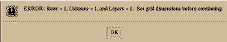Figure 15.3

1).

HEADNG(32)

Heading (#1)

2).

HEADNG(continued)

Heading (#2)

3).

NLAY

Layers

NROW

Rows

NCOL

Columns

NPER

Stress Periods

ITMUNI

Time Units: Pressing the appropriate menu toggle (Undefined, Seconds, Minutes, Hours, Days, Years) will set the value appropriately.

4).

IUNIT

Packages Used and Solver Used: By pressing the toggle button for each package, it may be selected and a unit number will by assigned that package. For the solver, select either the SIP or the SSOR package. The default unit numbers are as follows (These unit numbers must be honored):

BAS = 1
BCF = 11
DRN = 13
EVT = 15
GHB = 17
MT3D = 32
OC = 22
PCG2 = 23
RCH = 18
RIV = 14
SIP = 19
SOR = 21
WEL = 12

5).

IAPART

BUFF and RHS memory allocation

ISTRT

Starting Heads for Drawdown

6).

IBOUND

Boundary Conditions button: This calls the utility 2D integer array editor (See below, U2DINT).

7).

HNOFLO

Dummy NO-FLOW Head Value

8).

Shead

Starting Heads button: This calls the utility 2D real array editor (See below, U2DREL).

9).

PERLEN, NSTP, & TSMULT

Define Stress Periods button: Because there can be multiple stress periods a pop-up dialog is needed (Figure 15.4). An entry is needed for each stress period. If more then 10 stress periods are required, using the Previous and Next buttons will allow you to proceed through them. Length is equivalent to PERLEN, No. Steps to NSTP, and Multiplier to TSMULT.

Figure 15.4

Block Centered Flow:

Figure 15.5

1).

ISS

Steady-State Flag: Select either Steady-State or Transient.

IBCFCB

Cell-by-Cell Output: Output will be Not Saved, Saved to Standard Output, or Saved to File (A unit number will be automatically selected). If a filename is required, "Unknown" or a filename will be written in the Cell-toCell Filename text entry field. To enter a filename, type over the current entry or press the button Select. A dialog similar to that used in Figure 5.2 will be displayed. The default file extension is "*.ctc". If the CTC file already exists, the Convert to NCG button will convert the file to a NODE CENTERED GRID file (see Chapter 11. This option is not yet installed).

2).

LAYCON

Layer Types button: To enter the layer type for each layer the dialog shown in Figure 15.6 is used. Note, only the top layer can be unconfined (Type 1). If there are more than ten layers, use the Next and Previous buttons to define all layers.

Figure 15.6

3).

TRPY

Layer Anisotropy button: This calls the 1D utility array editor (See below, U1DREL).

4).

DELR

Width Along Rows button: This calls the 1D utility array editor (See below, U1DREL).

5).

DELC

Width Along Columns button: This calls the 1D utility array editor (See below, U1DREL).

6).

sf1, Tran, HY, BOT, Vcont, sf2, TOP

Layer Specifics button: These seven arrays can be fairly confusing to get correct. The dialog in Figure 15.7 based on layer type, layer position, and whether the simulation is transient or steady-state will determine which layers need to be specified. Arrays with a faded GRAY button are not needed, and cannot be specified. Arrays that need to be defined are identified with a RED button. Arrays that have been specified (not necessarily with meaningful information) and are needed, are colored GREEN. All of these arrays use the 2D utility array editor described below (See below, U2DREL).

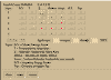Figure 15.7

Drain:

Figure 15.8

1).

MXDRN

This term is not entered by the user.

IDRNCB

Cell-by-Cell Output: Output will be Not Saved, Saved to Standard Output, or Saved to File (A unit number will bee automatically selected). If a filename is required, "Unknown" or a filename will be written in the Cell-to-Cell Filename text entry field. To enter a filename, type over the current entry or press the button Select. A dialog similar to that used in Figure 5.2 will be displayed. The default file extension is "*.ctc". If the CTC file already exists, the Convert to NCG button will convert the file to a NODE CENTERED GRID file (see Chapter 11, This option is not yet installed).

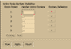Figure 15.9

2).

ITMP

Number Active Sections for stress period.

3).

Layer, Row, Col, Elevation, Cond

Sections Definition button for stress period: Pressing these button will pop-up the dialog shown in Figure 15.10. For each section, enter the appropriate Layer, Row, Column, Elevation, and Conductance. If there are more than ten sections, press the Next and Previous buttons as appropriate.

Figure 15.10

Evapotranspiration:

Figure 15.11

1).

NEVTOP

Evapotranspiration Application Location Option menu: Select applied to the Top Layer Only or Vertically Distributed.

IEVTCB

Print Cell to Cell Flow: Output will be Not Saved or Saved to File (A unit number will bee automatically selected). If a filename is required, "Unknown" or a filename will be written in the Cell-to-Cell Filename text entry field. To enter a filename, type over the current entry or press the button Select. A dialog similar to that used in Figure 5.2 will be displayed. The default file extension is "*.ctc". If the CTC file already exists, the Convert to NCG button will convert the file to a NODE CENTERED GRID file (see Chapter 11, This option is not yet installed).

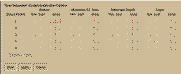Figure 15.12

2).

INSURF

Surface New or Last menu option for stress period.

INEVTR

Maximum ET Rate New or Last menu option for stress period.

INEXDP

Extinction Depth New or Last menu option for stress period.

INIEVT

Layer New or Last menu option for stress period.

NOTE: For each of the above options, the array for stress period 1 must be New.

3).

SURF

Surface button: This calls the 2D utility array editor (See below, U2DREL).

4).

EVTR

Maximum ET Rate button: This calls the 2D utility array editor (See below, U2DREL).

5).

EXDP

Extinction Depth button: This calls the 2D utility array editor (See below, U2DREL).

6).

IEVT

Layer button: This calls the 2D utility array editor (See below, U2DINT).

Figure 15.13

1).

MXBND

This term is not entered by the user.

IGHBCB

Cell-by-Cell Output: Output will be Not Saved, Saved to Standard Output, or Saved to File (A unit number will bee automatically selected). If a filename is required, "Unknown" or a filename will be written in the Cell-to-Cell Filename text entry field. To enter a filename, type over the current entry or press the button Select. A dialog similar to that used in Figure 5.2 will be displayed. The default file extension is "*.ctc". If the CTC file already exists, the Convert to NCG button will convert the file to a NODE CENTERED GRID file (see Chapter 11, This option is not yet installed).

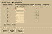Figure 15.14

2).

ITMP

Number Active GHB Zones for stress period.

3).

Layer, Row, Col, Head, Cond

GHB Zone Definitions button for stress period: Pressing these button will pop-up the dialog shown in Figure 15.15. For each section, enter the appropriate Layer, Row, Column, Head, and Conductance. If there are more than ten sections, press the Next and Previous buttons as appropriate.

Figure 15.15

MT3D:

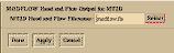Figure 15.16

Output Control:

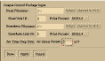Figure 15.17

1).

IHEDFM

Head Print Format menu list is used to select the file output format for heads. This is the same format list used in the utility package.

IDDNFM

Drawdown Print Format button is used to select the file output format for drawdowns. This is the same format list used in the utility package.

IHEDUN

Head Filename text field and Select button is used to select the output file to which heads will be saved. A dialog similar to that used in Figure 5.2 will be displayed. The default file extension is "*.head". If no file is selected (Press the Cancel button), heads will not be saved to a special file. If a non-zero Head Unit ID is specified, a filename must be given.

IDDNUN

Drawdown Filename text field and Select button is used to select the output file to which drawdowns will be saved. A dialog similar to that used in Figure 5.2 will be displayed. The default file extension is "*.dd". If no file is selected (Press the Cancel button), heads will not be saved to a special file. If a non-zero Drawdown Unit ID is specified, a filename must be given.

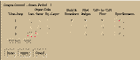Figure 15.18

2).

INCODE

The Output Code may be specified as the same as the Last time step (Not applicable for the first time step), as all layers treated the Same, or on a By-Layer basis.

IHDDFL

Head & Drawdown, when set to TRUE these terms will be saved.

IBUDFL

Print Budget, when set to TRUE the water budget will be saved.

ICBCFL

Cell-to-Cell, when set to TRUE will print data from the packages saving cell-to-cell information.

Figure 15.19

3).

Hdpr

Print Head, when true heads will be printed to standard output.

Ddpr

Print Drawdown, when true drawdowns will be printed to standard output.

Hdsv

Save Head, when true heads will be saved to the IHEDUN file.

Ddsv

Save Drawdown, when true drawdowns will be saved to the IDDNUN file.

NOTE: If the modmain interface is going to be used to create head or drawdown maps, head and drawdown must be printed to standard output. The standard output file is read my modmain to determine the result values.

PCG:

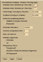Figure 15.20

1).

MXITER

Maximum Iterations per Time Step.

ITER1

Maximum Number of Inner Iterations.

NPCOND

Matrix Preconditioning Method. Modified Incomplete Cholesky (the default) should be used on scalar computers, and Polynomial should be used on vector computers.

2).

HCLOSE

Head Change Convergence Criteria.

RCLOSE

Residual Convergence Criterion.

RELAX

Relaxation Parameter. 1.0 is normally used, but 0.99, 0.98, or 0.97 will reduce the number of iterations required for convergence.

NBPOL

Maximum Eigenvalue method. This can be set to 2.0 or the program can estimate a value.

IPRPCG

Print-Out Interval for the PCG solver.

MUTPCG

Printing from Solver has several options: Unsuppressed, the number of Iterations are Printed, but Extremes Suppressed, or All printing is Suppressed.

IPCGCD

Cholesky Decomposition Calls. This should generally be set to zero.

Figure 15.21

1).

NRCHOP

Recharge Application Location Option menu: Select recharge applied to the Top Layer Only, Vertically Distributed (IRCH array), or Applied to Highest Active Cell.

IRCHCB

Print Cell to Cell Flow: Output will be Not Saved or Saved to File (A unit number will bee automatically selected). If a filename is required, "Unknown" or a filename will be written in the Cell- to-Cell Filename text entry field. To enter a filename, type over the current entry or press the button Select. A dialog similar to that used in Figure 5.2 will be displayed. The default file extension is "*.ctc". If the CTC file already exists, the Convert to NCG button will convert the file to a NODE CENTERED GRID file (see Chapter 11, This option is not yet installed).

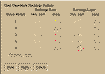Figure 15.22

2).

INRECH

Recharge Rate New or Last menu option for stress period.

INIRCH

Recharge Layer New or Last menu option for stress period.

NOTE: For each of the above options, the array for stress period 1 must be New.

3).

RECH

Recharge Rate button: This calls the 2D utility array editor (See below, U2DREL).

4).

IRCH

Recharge Layer button: This calls the 2D utility array editor (See below, U2DINT).

Figure 15.23

1).

MXRIVR

This term is not entered by the user.

IRIVCB

Cell-by-Cell Output: Output will be Not Saved, Saved to Standard Output, or Saved to File (A unit number will bee automatically selected). If a filename is required, "Unknown" or a filename will be written in the Cell-to-Cell Filename text entry field. To enter a filename, type over the current entry or press the button Select. A dialog similar to that used in Figure 5.2 will be displayed. The default file extension is "*.ctc". If the CTC file already exists, the Convert to NCG button will convert the file to a NODE CENTERED GRID file (see Chapter 11, This option is not yet installed).

Figure 15.24

2).

ITMP

Number Active Reaches for stress period.

3).

Layer, Row, Col, Stage, Cond, Rbot

Reach Definitions button for stress period: Pressing these button will pop-up the dialog shown in Figure 15.25. For each section, enter the appropriate Layer, Row, Column, Stage, Conductance, and Bottom. If there are more than ten sections, press the Next and Previous buttons as appropriate.

Figure 15.25

SIP:

Figure 15.26

1).

MXITER

Maximum Iterations per Time Step.

NPARM

Number of Iteration Parameters.

2).

ACCL

Acceleration.

HCLOSE

Head change Convergence Criteria.

IPCALC

Iteration Flag. This specifies whether the seed will be User Defined or Calculated at the Start of the Simulation.

WSEED

Seed. This parameter only needs to be set if IPCALC is set to Seed User Defined.

IPRSIP

Printout Interval.

Figure 15.27

1).

MXITER

Maximum Iterations per Time Step.

2).

ACCL

Acceleration.

HCLOSE

Head change Convergence Criteria.

IPRSOR

Printout Interval.

Figure 15.28

1).

MXWELL

This term is not entered by the user.

IWELCB

Cell-by-Cell Output: Output will be Not Saved, Saved to Standard Output, or Saved to File (A unit number will bee automatically selected). If a filename is required, "Unknown" or a filename will be written in the Cell-to-Cell Filename text entry field. To enter a filename, type over the current entry or press the button Select. A dialog similar to that used in Figure 5.2 will be displayed. The default file extension is "*.ctc". If the CTC file already exists, the Convert to NCG button will convert the file to a NODE CENTERED GRID file (see Chapter 11, This option is not yet installed).

Figure 15.29

2).

ITMP

Number Active Wells for stress period.

3).

Layer, Row, Col, Recharge

Well Definitions button for stress period: Pressing these button will pop-up the dialog shown in Figure 15.30. For each section, enter the appropriate Layer, Row, Column, and Recharge. If there are more than ten sections, press the Next and Previous buttons as appropriate.

Figure 15.30

Utility:

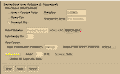Figure 15.31

REAL ARRAYS (U1DREL and U2DREL):
1).

LOCAT

Data Source (File/Constant): values for an array can be set as Array = Constant Value, or values may be read from an Unformatted File or a Formatted File. If the LOCAT does not define a constant, the Define Array button will be activated; RED indicates the array needs to be defined, and GREEN indicates it has been previously defined. To enter the array position values, press the Define Array button; it will pop-up the array editor discussed below. If LOCAT does not define a constant, a file Unit Number ID (positive only) must be specified. If the Unit Number ID does not match the unit number ID for the package being modified (See Packages:Basic - IUNIT section above), a Data Filename associated with the Unit ID also needs to be specified.

CNSTNT

If LOCAT is set to Array = Constant Value, the constant value should be entered in the Constant for Array text field. Otherwise, individual values are read for each array position, and the multiplier should be entered in the Multiplier text field.

FMTIN

Input FORTRAN77 FORMAT: This format is user specified for reading the data file. It must be a valid FORTRAN77 format for REAL numbers, and there must be an entry.

IPRN

Output FORTRAN77 FORMAT: This button allows the user to select the standard output file format for this array. For U1DREL the (10G12.4) format is the only valid format. For U2DREL, the valid formats can be selected from the menu list button. Valid formats are:

10G11.4
11G10.3
9G13.6
15F7.1
15F7.2
15F7.3
15F7.4
20F5.0
20F5.1
20F5.2
20F5.3
20F5.4
10G11.4

INTEGER ARRAYS (U2DINT):
1).

LOCAT

Data Source (File/Constant): values for an array can be set as Array = Constant Value, or values may be read from an Unformatted File or a Formatted File. If the LOCAT does not define a constant, the Define Array button will be activated; RED indicates the array needs to be defined, and GREEN indicates it has been previously defined. To enter the array position values, press the Define Array button; it will pop-up the array editor discussed below. If LOCAT does not define a constant, a file Unit Number ID (positive only) must be specified. If the Unit Number ID does not match the unit number ID for the package being modified (See Packages:Basic - IUNIT section above), a Data Filename associated with the Unit ID also needs to be specified.

ICONST

If LOCAT is set to Array = Constant Value, the constant value should be entered in the Constant for Array text field. Otherwise, individual values are read for each array position, and the multiplier should be entered in the Multiplier text field.

FMTIN

Input FORTRAN77 FORMAT: This format is user specified for reading the data file. It must be a valid FORTRAN77 format for INTEGER numbers, and there must be an entry.

IPRN

Output FORTRAN77 FORMAT: This button allows the user to select the standard output file format for this array. For U2DINT, the valid formats can be selected from the menu list button. Valid formats are:

10I11
60I1
40I2
30I3
25I4
20I5

NOTE and WARNING: The standard release of MODFLOW does not support the PCG2 solver or MT3D. If you want to use these packages, you need to update the software yourself, or download the copy of MODFLOW released with UNCERT (See Chapter 2, the Acquiring Software section).

Now:

NOTE: MODFLOW is executed with a system call; as a result modmain cannot independently determine when MODFLOW is done or if there has been a problem. The standard MODFLOW messages, however will still be printed to the xterm window that launched modmain. When MODFLOW is complete, "STOP" will be printed in the xterm window.

[TOP] [SYNTAX]

NOTE: These options are not available until MODFLOW has been run, using the Run:Now menu-bar option.

WARNING: Because there is currently no error checking on whether MODFLOW completed successfully, modmain may try to map head values that do not exist. Before you try to make a grid or block file, examine the file to insure it has completed successfully.

MODFLOW Output File:

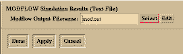Figure 15.32

Figure 15.33

Drawdown/Head - Contoured Surface:

Figure 15.34

NOTE: The X-Z and Y-Z Plane options are not installed.

NOTE: If a cell has gone dry, MODFLOW will mark it by giving it a head value of HNOFLO (Basic Package). When creating the X. Y, Z, head value data file, any cells with heads greater than HNOFLO will be considered dry and not included in the data file. When a cell value is discarded, a WARNING message identifying the cell position will be displayed in the log-status window.

NOTE: Because grid is an independent program module, it must be terminated separately from modmain. Also, once grid is open, modmain can no longer inform it what files to load. If the Grid Data button is pressed repeatedly with the Create XYZ Data File and Grid option set, there will be multiple instances of grid running using up computer memory. It is therefore best to 1) quit grid after each grid data file is created, or 2) to set the Run Gridding Program option to Create XYZ Data File Only. Once the XYZ data file is created, it is a simple matter to load the new XYZ data file with grid.

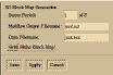Figure 15.35

NOTE: If a cell has gone dry, MODFLOW will mark it by giving it a head value of HNOFLO (Basic Package). When creating the X. Y, Z, head value data file, any cells with heads greater than HNOFLO will be considered dry and not included in the data file. When a cell value is discarded, a WARNING message identifying the cell position will be displayed in the log-status window.

NOTE: Cells with values outside the minimum and maximum head/drawdown will not be display when viewed using block.

NOTE: Because grid and block are independent programs module, they must be terminated separately from modmain. Also, once open, modmain can no longer inform them what files to load.

[TOP] [SYNTAX]

[TOP] [SYNTAX]

[TOP] [SYNTAX]

NOTE: Only one help window may be open at a time.

Help files are editable ASCII data files; for further information see Appendix D.

[TOP] [SYNTAX]

Figure 15.36

Array:

Print Setup:

Print:

Quit:

Edit:

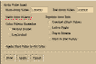Figure 15.37

The color palette, is set linearly from the minimum to the maximum data values in the array (Normal Scaled Color Palette Gradation). Because many parameters very over several orders of magnitude (e.g. hydraulic conductivity - clay = 10-5 ft/day, gravel = 103 ft/day), however, a linear color scale will hide much of the detail. For this reason, the color scale can be Log Scaled (Note, any values <= 0.0 will be set to BLACK). If array value range has been changed, pressing the Refit Color Palette button will rescale the color palette.

To enter new values in the array, enter the desired value(s) in the Start Array Value and End Array Value (optional) text fields. Pressing the Apply Start Value to All Cells will apply the value in the Start Array Value text field to all the cells in the array; this is a quick way to initialize the array to a given value. Values may also be entered into the array using the mouse. When the left mouse button is held down and the mouse is moved, a small rectangle is created. When the mouse button is released, all cells that are under or within the rectangle will be reset based on the current Populate Rule. Individual cells can be changed by pointing at a cell and pressing and releasing the left mouse button. The rules are detailed below:

Constant (Start Value):

All cells marked, will be set to the value in the Start Array Value text field.

Left to Right:

When marking the rectangle, cells on the side of the rectangle where the mouse was first pressed will be assigned the Start Array Value. Those on the other side will be assigned the End Array Value. Cell in-between, will be defined based on the linear distance of the middle of the cell to the distance between the middle of the right and left most selected cells (Figure 15.38a).

Figure 15.38a

Top to Bottom:

When marking the rectangle, cells on the side of the rectangle where the mouse was first pressed will be assigned the Start Array Value. Those on the other side will be assigned the End Array Value. Cell in-between, will be defined based on the linear distance of the middle of the cell to the distance between the middle of the top and bottom most selected cells (Figure 15.38b).

Figure 15.38b

Start to End Vector:

When marking the rectangle, the cell in the corner of the rectangle where the mouse was first pressed will be assigned the Start Array Value. The cell in the opposite corner will be assigned the End Array Value. Cell in-between, will be defined based on the linear distance of the middle of the cell starting cell to the middle of the ending cell (Figure 15.38c & 15.38d).

Figure 15.38c and Figure 15.38d

A combination of the rules can be used to create more complex arrays as shown in Figure 15.38e or Figure 15.36.

Figure 15.38e

[TOP]

To run the correct or actual solution, run modmain, and load the project file f93cor.prj (Use the Project:Open Project menu-bar option). Opening the project will load several files into the application. These files are display in the log/status window and are also listed below:

f93.bas : BASIC INPUT PACKAGE
f93cor.bcf : BLOCK CENTERED FLOW INPUT PACKAGE
f93.oc : OUTPUT CONTROL INPUT PACKAGE
f93cor.rch : RECHARGE INPUT PACKAGE
f93cor.riv : RIVER INPUT PACKAGE
f93.sip : SIP INPUT PACKAGE

When modmain reads in f93.bas, it recognized that the BCF, OC, RCH, RIV, and SIP packages are also required. These are defined by the Packages Used and Solver Used toggles and toggle menu (IUNIT variables, Figure 15.2). If you pull down the Packages menu-bar you will note that all of the above packages are highlighted in GREEN. This means that all of the required packages are defined, and MODFLOW can be run.

WARNING: A package can be defined, without necessarily having reasonable entries.

To execute MODFLOW with these modules, select the Run:Now menu-bar option. A pop-up dialog will appear (similar to Figure 5.2) asking for the name of a script file. A script file is simple an ASCII text file with instructions the UNIX operating system can understand and execute. Select f93cor.csh. Modmain will determine what files are needed, build the script file, and tell the UNIX operating system to execute the script. In the log/status window a message will be printed:

Executing MODFLOW
SYSTEM CALL: $PWD/f93cor.csh &
NOTE: WAIT for "STOP" to appear in the xterm text window before continuing.

Once MODFLOW is complete, modmain can be used to view the results. To view the text file, select the View:MODFLOW output file menu-bar option. Press the View Output Filename button (Figure 15.32) and the standard output file generated by MODFLOW will be displayed (Figure 15.33). To make a contour map of the model head results, select the View:as Contoured Surface menu-bar option. The model was steady- state, so there is only one stress period; it was also, only a one layer X-Y plane model, so the default values shown in Figure 15.34 are correct. To create a data file containing the X, Y coordinates and head value for each cell, press the Grid Data button.

NOTE: In the log-status window, there are several WARNINGS. For six cells, the head value was 1.0e30! This is how MODFLOW indicates the cell went dry. These values are not included in the data set, because they have no real meaning with regard to the water table level at those locations.

Once the file has been created, grid (Chapter 10) is called, and several parameters are passed to that application. The most important are the X, Y, head value file name, and the number of columns and rows to use to build the grid (By default, twice the MODFLOW rows and columns plus 1 are used; this reduces some of the problems with the inverse-distance gridding algorithm honoring the MODFLOW results). For this example, it is sufficient to select Method:Calculate from the grid menu-bar. When the grid is calculated, select View:Contour Map from the grid menu-bar, and save the file to junk.srf (See Chapter 10 for further detail on using grid). Once the file is saved, the grid file will be passed to contour (Chapter 11) and displayed. A map similar to Figure 15.39 will be displayed. In addition to the normal features of a contour map, the areas outside of the flow region have been blanked out (description file = f93.blk) and the location the calculated heads are marked by "+" symbols (description file = junk.dat; this is the X, Y, head value data file created by modmain, and used by grid to generate the displayed grid file). These filenames are specified in the contour preference file, "contour.prf."

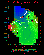Figure 15.39

NOTE: In the lower-left portion of the map area, where the regular grid would imply that there should be some head measurement, the "+" symbol is missing. These are some of the locations where the cells went dry.

For further details on using contour, refer to Chapter 11.

[TOP]

Syntax: modmain [project file name]

NOTE: Parameters in [] brackets are optional.

[TOP]

Project File:

Associated Files
MODFLOW Package Files (Basic Package file first)
Cell-to-Cell Files

For each file, three pieces of information are needed: 1) the files unit ID, 2) the files name, and 3) the unit ID of the owning package (e.g. block.ctc might be owned by the Block Center Flow Package, unit 11). A sample file might look like:

41 starting_head.dat 1
42 hyd_cond.dat 11
1 sample.bas 1
11 sample.bcf 11
43 block.ctc 11

Script File:

\cp sample.bas ----- fort.1
\cp sample.bcf ----- fort.11
\cp starting_head.dat -----fort.41
\cp hyd_cond.dat -----fort.42
modflow > mod.out
\rm ----- fort.1
\rm ----- fort.11
\rm ----- fort.41
\rm ----- fort.42
\mv fort.42 ----- block.ctc

[TOP]