


Sisim is a graphical user interface (GUI) for sisim3d an indicator kriging and conditional stochastic simulation program for discrete data (non-continuous data: e.g. clay, sand, gravel) developed at Stanford University by Gómez-Hernández and Srivastava (ISIM3D, 1990) and modified at the Colorado School of Mines by McKenna (1994) to utilize soft data (Discussed in Chapter 8 Mathematics section). Up to eight indicators can be modeled in a single simulation. In its basic form sisim3d can be awkward to use, particularly when many simulations are required based on varying semivariogram models. This interface assists the user in handling data files, input parameters, coordinating multiple simulation, tasking jobs to other computers, calculating simulation statistics, and visualizing results.
This chapter goes into the details of using sisim as an interface for sisim3d. The documentation supplied with sisim3d is limited, and this program will try to clarify some of the points.
The sisim application is composed of two sections; the main menu-bar and the log-status text area. The menu-bar is used to select all sisim commands, and the log/status area is used by the program to report important messages and results. The log/status area may also be used to personally enter important comments or notes; it is a simple text editor.
Open Project:
Project:Open Project generates a pop-up dialog which allows the user to select an
existing project file. The dialog functions as the File:Open dialog in Figure 5.2
(Plotgraph - Chapter 5). The default project file name extension, though is "*.prf".
View Project:
Project:View Project pops up a simple screen editor with the last saved version of
the opened or saved project file.
Save Project:
Project:Save Project saves the names of the appropriate files and computers, and
various simulation parameters to the named project file (See Sisim Output Data File
section for file format). If no project file name exists, the user will be queried for a file
name. The dialog functions as the File:Open dialog in Figure 5.2, except that the file
name does not have to pre-exist. For a description of how to use the dialog, see the
File:Save section in Chapter 5.
Save Project as:
Project:Save as is used to save the project to a new file. A pop-up dialog similar
to that used in File:Open (Figure 5.2) is created. This option is the same as Project:Save
Project except that a project file name must be selected.
Quit:
File:Quit terminates the program, but if additions have been made to the project
or any project sub-files, the user will first be queried to supply a file to save the changes
in.
Quit Without Saving:
File:Quit Without Saving terminates the program regardless of any additions to
the project. Once pressed there is no option to change your mind.
Configuration:
The configuration file specifies several limiting characteristics about the
simulation calculation. Features present in the data set can be temporarily turned off
for testing or debugging.
Open Configuration:
Packages:Configuration:Open Geometry generates a pop-up dialog which allows
the user to select and existing configuration file. The dialog functions as the File:Open
dialog in Figure 5.2 (Plotgraph - Chapter 5). The default project file name extension,
though is "*.set".
View Configuration:
Packages:Configuration:View Geometry pops up a simple screen editor with the
last saved version of the opened or saved geometry file.
Save:
Packages:Configuration:Save saves the current configuration parameter
specifications to the configuration file (See Sisim Input Data File section for file format).
If no geometry file name exists, the user will be queried for a file name. The dialog
functions as the File:Open dialog in Figure 5.2, except that the file name does not have
to pre-exist. For a description of how to use the dialog, see the File:Save section in
Chapter 5.
Save as:
Packages:Configuration:Save as is used to save the geometry to a new file. A
pop-up dialog similar to that used in File:Open (Figure 5.2) is created. This option is
the same as Project:Save Project except that a project file name must be selected.
Modify:
Packages:Configuration:Modify generates the pop-up dialog shown in Figure
14.2. This dialog allows the user to define several things about what data is treated in
the simulation. These generally effect the speed with which the simulation will run.
The options can also be set, so that the simulation will ignore certain data. This saves
having to build new data sets. The Grid Dimension can be either 2D or 3D. Hard Data
Only can be used; if the data set includes soft data, it will be ignored. No Type B Data
is in the data set. If this is set, it will improve the efficiency of some calculations.
Coarse Simulation Only allows only the first pass of the simulation to be run. Sisim3d
normally uses two passes to create a simulation grid. One pass makes a coarse grid,
and the second pass makes a finer grid using the results from the first pass. Often it is
worth running the coarse grid only on the first simulation. This allows the user to fine
basic logic errors, without having to wait for a full simulation to complete.
Data:
The input file containing the X, Y, Z, and indicator data must be read in before
any other operations can be done (Project files can be opened, because they open a data
file). This is because other portions of the program depend on the extents of the data
set.
Select Data File:
Packages:Data:Select Data File generates a pop-up dialog which allows the user
to select and existing data file. The dialog functions as the File:Open dialog in Figure
5.2 (Plotgraph - Chapter 5). The default project file name extension, though is "*.dat".
View Data File:
Packages:Data:View Data File pops up a simple screen editor with the last saved
version of the opened data file.
Geometry:
The geometry file in sisim3d specifies details about the model grid, and how
search parameters for finding data points near the location being evaluated. The
following options allow the user to load and edit an existing geometry file or create a
new file.
Open Geometry:
Packages;Geometry:Open Geometry generates a pop-up dialog which allows the
user to select and existing geometry file. The dialog functions as the File:Open dialog in
Figure 5.2 (Plotgraph - Chapter 5). The default project file name extension, though is
"*.geom".
View Geometry:
Packages;Geometry:View Geometry pops up a simple screen editor with the last
saved version of the opened or saved geometry file.
Save:
Packages;Geometry:Save saves the current geometry parameter specifications to
the geometry file (See Sisim Input Data File section for file format). If no geometry file
name exists, the user will be queried for a file name. The dialog functions as the
File:Open dialog in Figure 5.2, except that the file name does not have to pre-exist. For
a description of how to use the dialog, see the File:Save section in Chapter 5.
Save as:
Packages;Geometry:Save as is used to save the geometry to a new file. A pop-up
dialog similar to that used in File:Open (Figure 5.2) is created. This option is the same
as Project:Save Project except that a project file name must be selected.
Modify:
Packages;Geometry:Modify generates the pop-up dialog shown in Figure 14.3.
This dialog is used to specify all of the parameters needed for the model geometry, and
the search parameters required to locate appropriate data points when evaluating a
location. Parameters that need to be defined are: (1) the X, Y, and Z coordinates model
grid Origin; (2) the size of each node (Delta X, Y, Z), coarse and fine;
(3) the number of Nodes in each direction; (4) which nodes will be evaluated during this simulation (From-To -- this option is used to debug sub-regions of the model); (5) the shape and size of the search ellipsoid (data points within the search ellipsoid around the node being evaluated will be used); and (6) details about the search direction rotation. Details about the extents of the data set are also provided.
The Direction Cosine's and the Rotation Flag define the orientation of the search ellipsoid, and are important to define when the semivariogram models are not isotropic. Under isotropic conditions the Direction Cosine matrix is an identity matrix (1's on the diagonal, 0's elsewhere), and the No rotation Rotation Flag is used. For two-dimensional and some three-dimensional data sets it may be adequate to do a rotation about a single axis; with more complicated models though it may be necessary to perform a General rotation about all three axes. The values for the Direction Cosine matrix can be calculated by pressing the Calculate Direction Cosine button. This will create the pop- up dialog shown in Figure 14.4. Rotation angles should be entered in degrees. You can also enter the direction cosine values directly. Depending on the Rotation Flag, they are based on the following matrix's (Foley et al, 1990):
 (14-1)
 (14-2)
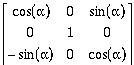 (14-3)
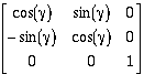 (14-4)
General rotation
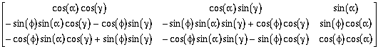 (14-5)
Semivariogram:
With sisim there are two methods of defining the model semivariograms, Single
and Latin-Hypercube Solutions. Single is the most common approach. Latin-Hypercube
Solutions are used only when the threshold or indicator semivariograms have been
calculated using the jackknifing option in vario (Chapter 8) and the latin-hypercube
sampling option in variofit (Chapter 9). This option, on a practical basis is only applied
when there is very little hard and soft data.
When using indicator semivariograms there will be the same number of indicators as semivariogram models. When using threshold semivariograms there will be one less semivariogram model then the number of indicators.
Single:
Packages:Single model semivariograms and needed for each threshold/indicator
in the indicator model, and there are one fewer thresholds than indicators. This section
allows the user to open, save, and edit the sisim3d semivariogram file. Note that one
file contains all of the threshold model semivariogram definitions.
Semivariogram:Single:Open Semivariogram generates a pop-up dialog which allows the user to select and existing semivariogram file. The dialog functions as the File:Open dialog in Figure 5.2 (Plotgraph - Chapter 5). The default project file name extension, though is "*.var".
Packages:Semivariogram:Single:View Semivariogram pops up a simple screen editor with the last saved version of the opened or saved semivariogram file.
Packages:Semivariogram:Single:Save saves the current semivariogram parameter specifications to the semivariogram file (See Sisim Input Data File section for file format). If no semivariogram file name exists, the user will be queried for a file name. The dialog functions as the File:Open dialog in Figure 5.2, except that the file name does not have to pre-exist. For a description of how to use the dialog, see the File:Save section in Chapter 5.
Packages:Semivariogram:Single:Save as is used to save the semivariogram to a new file. A pop-up dialog similar to that used in File:Open (Figure 5.2) is created. This option is the same as Project:Save Project except that a project file name must be selected.
Packages:Semivariogram:Single:Modify first generates the pop-up dialog shown in Figure 14.5. This dialog allows the user to define the Solution Type (Threshold, the must commonly used, or Indicator), the Number of Thresholds/Indicators that will be used in the simulation and therefore the number of required semivariogram models. It also allows the user to specify which Threshold Semivariogram is to be edited. Under the Cumulative Distribution Function the Threshold cutoff (values less then this threshold and greater than lesser thresholds will be evaluated with this semivariogram model) and the Prior cdf (cumulative distribution function) must be defined. The Prior cdf represents the decimal percent of the data set with values less than the cutoff (histo (Chapter 6) can be used to calculate these values). The semivariogram model definition allows up to four nested structures (sisim3d allows more, and the data file can be edited independently, but it is felt that more than this many structures is unrealistic, except in the most unusual circumstances). For each structure, Range, Sill, Semivariogram Model, and X, Y, and Z Anisotropy's must be defined. The model Nugget must also be defined, and if a Power model is used, C Maximum must be defined. The model specifications are aligned vertically from left to right (1, 2, 3, 4). Note, if higher order nests are not used, be sure to mark None for the Semivariogram Model type.
When calculating the anisotropy's assume the major semivariogram model axis is the X-axis, and the Y or Z-axis is the minor axis. The X anisotropy's will then be 1.0, and the Y and Z anisotropy's will be the X anisotropy divided by the Y or Z anisotropy (With this approach, anisotropy's will be greater or equal to 1.0). Using this approach, the model semivariogram must also be rotated accordingly. The Direction Cosine matrix should be defined using equations 14-1, 14-2, 14-3, 14-4 and 14-5 or the dialog shown in Figure 14.4.
Latin-Hypercube Solutions:
When there is not enough data to adequately define a model semivariogram,
latin-hypercube sampling can be used to define a range of reasonable model
semivariograms (See variofit Mathematics section, Chapter 9). Simulations can then be
run on each model semivariogram for each threshold.
Because of the complexity of this data set, it is best to let variofit (Chapter 9) build the data file. Refer to Chapter 9 for the data file format if interested.
Packages:Semivariogram:Latin-Hypercube Solutions:Open Semivariogram generates a pop-up dialog which allows the user to select and existing latin-hypercube semivariograms file. The dialog functions as the File:Open dialog in Figure 5.2 (Plotgraph - Chapter 5). The default project file name extension, though is "*.lhc".
Packages:Semivariogram:Latin-Hypercube Solutions:View Semivariogram pops up a simple screen editor with the last saved version of the opened or saved latin- hypercube semivariograms file.
Uncertainty:
The uncertainty file describes the probability distributions for the soft data.
Even if no soft data is used still file is required, though it is very simple.
Select Uncertainty File:
Packages:Uncertainty:Select Uncertainty File generates a pop-up dialog which
allows the user to select and existing uncertainty file. The dialog functions as the
File:Open dialog in Figure 5.2 (Plotgraph - Chapter 5). The default project file name
extension, though is "*.dat".
View Uncertainty File:
Packages:Uncertainty:View Uncertainty File pops up a simple screen editor with
the last saved version of the opened data file.
If a Starting Simulation Number other than 1 is used, the Random Number Seed will be incremented accordingly. This allows simulations to be rerun individually without having the user calculate the appropriate seed. After the simulations are run, the simulation results will be saved to files based on the Output File Name selected here. If "example.junk" is specified, for 5 simulations, starting at simulation 5. The output files would be named:
	Coarse Grid			Fine Grid
	example.junk.cor.5.sim		example.junk.5.sim
	example.junk.cor.6.sim		example.junk.6.sim
	example.junk.cor.7.sim		example.junk.7.sim
	example.junk.cor.8.sim		example.junk.8.sim
	example.junk.cor.9.sim		example.junk.9.sim
These files are saved in NODE CENTERED GRID format (See Chapter 11, Data File Format section).
Mode:
Network:Mode allows the user to select between Single computer mode (no
network connection required) or between Multiple networked computer mode.
Select Computer List:
Network:Select Computer List generates a pop-up dialog which allows the user to
select and existing file which specifies what computers are available to be used. This
list does not specify that any of the listed computers will be used. The dialog functions
as the File:Open dialog in Figure 5.2 (Plotgraph - Chapter 5). The default project file
name extension, though is "*.net".
View Computer List:
Network:View Computer List pops up a simple screen editor with the last opened
version of the computer list file.
Select Computers:
Network:Select Computers generates the pop-up dialog shown in Figure 14.7.
This option is only valid when sisim is in the Multiple Mode. This shows a list of the
computers available for use (The list comes from the loaded *.net file. It is the user's
responsibility to insure this file is correct). By default no computers are used. Select
the computers which are available. All computers on the list can be marked, but there
are several thing to keep in mind:
When using other computers, consider your job priority versus that of other user's!
Model Summary:
Model Summary is used to determine the distribution frequency, and frequency
variance and standard deviation for each indicator in a single simulation, or in all on
the simulations.
Individual Simulation:
Statistics:Model Summary:Individual Simulation will generate the pop-up dialog
in Figure 14.9. This dialog will allow the user to specify which simulation series is of
concern and which simulation in the series will be evaluated. The statistics when
calculated (Press View Statistics) will be display in a pop-up dialog similar to Figure
14.10. The statistics can also be echoed to the log/status window if the Print Statistics
to Log/Status Window toggle is set. In this dialog, for each indicator, the cell count and
frequency of occurrence is displayed. The cumulative count and frequency, mean,
median, and mode are also displayed.
All Simulations:
Statistics:Model Summary:All Simulation will generate the pop-up dialog in Figure
14.11. This dialog will allow the user to specify which simulation series is of concern,
the output file name prefix, and which simulations (from-to) in the series will be
evaluated. The statistics when calculated (Press Calculate Map & View Statistics) will
be display in a pop-up dialog similar to Figure 14.12. The statistics can also be echoed
to the log/status window if the Print Statistics to Log/Status Window toggle is set. In
this dialog, for each indicator, the frequency of occurrence, variance, and standard
deviation is displayed. The cumulative frequency, mean, median, and mode are also
displayed. Calculated and created with the statistics, are several maps. The Probability
Map Files specify the calculated probability that the given indicator will be present in
each cell (Figures 14.13a, 14.13b, and 14.13c). The Certainty Map File indicates the
maximum probability of occurrence of any indicator at every cell location (Figure 14.14).
This map highlights zones of good and poor data control. It, however cannot be used to
identify what indicator is present. The final map created is the Best-Guess Map. This
map will determine which indicator is the most probable at each cell location, and
assign the appropriate indicator value (Figure 14.15). If enough simulations were run,
this map should appear nearly identical to an indicator kriged map which always
selected the best-guess (0.50) cdf indicator.
Figure 14.13a,
Figure 14.13b and
Figure 14.13c
Figure 14.17a and
Figure 14.17b
To run the correct or actual solution, run sisim, and load the project file three.prj (Use the Project:Open Project menu-bar option). Opening the project will load several files into the application. These files are display in the log/status window and are also listed below:
	three.dat	: DATA PACKAGE
	three.geom	: GEOMETRY PACKAGE
	three.var	: SEMIVARIOGRAM PACKAGE
	three.set	: CONFIGURATION PACKAGE
	three.unc	: UNCERTAINTY PACKAGE
Next, pop-up the Simulator:Modify dialog (Figure 14.6). The maps shown were based on 100 simulations, but those runs took several hours. Just select three simulations. Everything else in the dialog can stay the same. Even these three simulations will take some time. To speed the process, we can just run the coarse simulations. To go this, bring up the Packages:Configuration:Modify dialog (Figure 14.2), and Set Coarse Simulation Only to TRUE. Next, save the file to a new file (Packages:Configuration:Save as). Any file name will do; junk.set would be good.
At this point, everything is set to run in single computer mode. To execute sisim3d with these modules, select the Run:Now menu-bar option. Sisim will determine what files are needed, and tell the UNIX operating system to execute sisim3d. In the log/status lots of messages will be printed regarding the status of the simulation executions. Eventually, the follow message will appear:
Once Sisim is complete, statistics and maps for each simulation and all simulations can be created. To view the statistics for an individual simulation, select the Statistics:Model Summary:Individual Simulation option. A dialog similar to Figure 14.9 will be created. Set the Series prefix to junk.cor (We only ran the coarse portion of the simulation). When the View Statistics button is pressed, another dialog will appear (Figure 14.10). This dialog summarizes the statistics for simulation one (or which ever one was selected). To view the statistics for all three simulations, select the Statistics:Model Summary:All Simulations option. A dialog similar to Figure 14.11 will be created. Set the Last Simulation to 3, and press the Calculate button at the bottom of the dialog. The summary statistics will be displayed in a new dialog (Figure 14.12). To examine the Probability, Certainty, or Best-Guess Map, you just need to press the Block, Contour or Surface buttons. These will start the appropriate program with the appropriate file. To view an individual simulation, select the desired simulation number from the View:Map dialog (Figure 14.16).
Syntax: sisim [project file]
Syntax:
Meaning of flag symbols:
NOTES:
If no entry is required for flag, flag command executed.
Flag Definitions:
| -client | = | hostname of computer running sisim3d | default = " " | ||
| -cou | = | coarse simulation file | default = "sisim3d.cou" | ||
| -data | = | X-Y-Z-indicator data file | default = "sisim3d.dat" | ||
| -geom | = | debug file | default = "sisim3d.dbg" | ||
| -geom | = | geometry file | default = "sisim3d.geom" | ||
| -help | = | give this help menu | |||
| -out | = | output file | default = "sisim3d.out" | ||
| -seed | = | simulation random seed | default = "-1" | ||
| -serv | = | specifies server type | default = 0 | ||
|
|||||
| -set | = | configuration setup file | default = "sisim3d.set" | ||
| -sim | = | simulation number | default = 1 | ||
| -unc | = | soft data uncertainty file | default = "sisim3d.unc" | ||
| -var | = | semivariogram file | default = "sisim3d.var" |
Project Files:
The project tells sisim what file need to be loaded for input, what file names will
be for output, the seed, the seed increment, the starting simulation number, the
number of simulations that will be run, and the list of computers that will be used for
the model calculations. The format is specified below:
An example file is three.prj.
Configuration Files (sisim3d):
The configuration file specifies information about the grid dimensions, what type
of data will be used, and whether both the fine and coarse simulation grids will be
made. The format is specified below:
Data Files (sisim3d):
The data file specifies the number of hard conditioning data points, and the X,
Y, and Z coordinate, and value for each conditioning point. This is a standard sisim3d
data file. The format is specified below (This is the file format given in sisim3d's
smain22.c program module):
An example file is sisim3d.dat.
Geometry Files (sisim3d):
The geometry file contains the following information in the format specified
below (This is the file format given in sisim3d's main.c program module):
NOTE:
record 5:
rotation = 0, (no rotation; identity matrix)
rotation = 1, (rotation around the x axis)
rotation = 2, (rotation around the y axis)
rotation = 3, (rotation around the z axis)
rotation = 4, (general rotation)
record 13:
An example file is three.geom.
Semivariogram Files (sisim3d):
The semivariogram file specifies the parameters for each semivariogram at each
threshold. This is a standard sisim3d semivariogram file. The format is specified below
(This is the file format given in sisim3d's main.c program module):
NOTE:
record 2:
1: spherical
2: exponential
3: gaussian
4: power
record 8:
NOTE:
record 10:
records 2 to 15 are repeated for each of the remaining indicator variables.
An example file is three.var.
Uncertainty Files (sisim3d):
The uncertainty file specifies the probability distributions for the soft data (This
is the file format given in sisim3d's main.c program module):
(records 11 thru 18 are repeated num_C times)
An example file is three.unc.
Latin-Hypercube Semivariogram Files:
Refer to the variofit Output Data File Format section in Chapter 9.
An example file is well.aniso.4.lhc.
Computer List Files:
The computer file list, is simply a list of the internet names of computers
available for use. The full internet name can be used, or if it is a local machine, only
the local name is required (e.g. pikes.mines.colorado.edu equals pikes in a local
network). The file format is simply a list of the computer name, with one name per line.
An example file is computer.net.
.netrc:
The .netrc file is a UNIX system which allows a user application to run processes
on remote computers. This file must be on each computer used in the user's login
directory. This file is a list of computer names, and the user name, and the user
password for each computer. The file format is:
One entry is needed for every computer. An example file might look like:
WARNING: This file has the user password spelled out; it is not encrypted! Make sure that file protections are set for this file so that only the user can read it! Also note, anyone with root privilege can read this file regardless of the privileges!
Debug:
Depending on the debug level set, sisim3d will list out more or less detail about
the simulation calculations. The output is in a free format.
Block & sisim3d Output:
Sisim model simulation output is in block format. Refer to the Setting up the
Input File-Equal Dimensions section in Chapter 13.
Once the semivariograms have been developed, the sample data can be indicator kriged or Bayesian kriged at each cutoff. The process of determining the weight of sample values at the point being estimated is identical to that used in ordinary kriging whether blocks or points are being evaluated:
where wi and bi are weights, gc is the global distribution, F(gc) and Z*(x) are kriged estimates, and the summations are from 1 to the number of data points (n). Note that these are basically the same equations except that equation 14-7 is multiplied by the indicator value (0 or 1). To determine the indicator value at the prescribed point, a cumulative distribution function (cdf) is developed. In Figure 14.18, a simple example is shown for defining the cdf for an individual block. In this case, five samples are equally distant from the block (and within the range of influence), and therefore the weights are equal (w1 = w2 = w3 = w4 = w5 = 0.20). Cutoffs were set at 0.02, 0.10, 0.13, and 0.26. Only one point is less than or equal to the first cutoff (0.02) so there is a 20% probability the value at the point is less then 0.02, 40% probability of being less then 0.10, 60% probability of being less then 0.13, and an 80% probability of being less then 0.26.
From this point several tacks may be taken in evaluating the indicator data based on the cdf; 1) maps can be made defining the best estimate of parameter values (value defined equal the value equal to the 50% probability), 2) maps can define the probability that the value of a parameter is above or below some specified level, 3) maps can define the parameter value above or below given a specified probability, or 4) realization maps can be made where the values are determined by randomly selecting the indicator for each location from the cdf; this last option is a stochastic simulation.
Stochastic Simulation:
There is a distinct difference between ordinary kriging (and most other
estimation methods) and Bayesian Kriging with conditional simulation. Most
techniques tend to average or smooth the data to achieve a best estimate of conditions
between measured points. Conditional simulation provides a means of representing the
variability of observed in nature, while still honoring the field data (Figure 14.19).
Conditional simulation does not produce a best estimate of reality, rather it yields
equiprobable models with characteristics similar to those observed in reality.
The process of stochastic simulation, described by Gómez-Hernández and Srivastava (1990), takes advantage of cdf's determined by indicator kriging, and Monte- Carlo techniques. To generate an individual realization, or a stochastic simulation, a search grid is selected (Figure 14.20). Starting with the first indicator range (e.g. clay), grid blocks at hard data locations are defined as "1" (clay) or another indicator type (e.g. "2" = sand, "3" = gravel; in kriging calculations these values are treated as "0" if another indicator is being evaluated or as "1" if it is the indicator currently under consideration). At soft data locations, blocks are defined with the aid of a random number generator. A random number between 0.0 and 1.0 is generated. If the value is less than the probability the property exists, the location is defined as the given indicator type; if the random number is greater than the probability, the indicator exists, then the block is defined with an alternate indicator type (for example, if the location has a 70% probability of being clay, 20% sand, and 10% gravel, and a random number of 0.87 is generated, the location is defined as sand, "2"). Because many realizations are created, at this location, clay will be present about 70% of the time, sand 20%, and gravel 10%. When all the hard and soft data are entered, a random starting location within the model grid is selected and the location is kriged based on the indicator cdf and a new random number. The cdf, at this point is based only of the hard and soft data, where the soft data are treated as hard or exact (It has been defined and is now known). If the random number is less then the probability, the indicator value exists, a "1" is assigned (i.e. clay is present at the grid location), otherwise a "0" is defined (another indicator is present). Next, another random grid location for which an indicator has not been defined is considered, and its indicator value is determined based on the hard and soft data, and the previously kriged indicators at other locations (now considered a hard data values for the remainder of the simulation). This process of selecting random grid locations and kriging them, based on the hard, soft, and previously kriged data, is continued until all grid locations are defined and a map of "1's" (clay) and "0's" (not clay) is created. The next indicator range is then selected (sand) and all the locations still containing "0's" are re-kriged (here the cdf is based only on the possibility the parameter value is sand or gravel). This re-kriging process is repeated until all the indicator ranges have been evaluated and the map is composed of all "1's."
To create another realization, the process is repeated. Soft data locations are re- evaluated, cdf's are calculated, a new random path through the grid is selected and each grid location is re-kriged and simulated. Alternative realizations can be created following this process until the desired number of simulations are created.
Each realization honors the statistics of the original data, and has equal probability of existing. These realizations can be used as maps of parameters for modeling of the site.
Gómez-Hernández, J.J. and R.M. Srivastava, 1990, ISIM3D: An ANSI-C Three Dimensional Multiple Indicator Conditional Simulation Program, Computers in Geoscience, Vol.. 16, No. 4, pp. 395-440.
McKenna, S.A., 1994, Utilization of Soft Data for Uncertainty Reduction in Groundwater Flow and Transport Modeling, Ph.D. Dissertation, Colorado School of Mines.