AAPG '98 Annual Convention, Advances in Geostatistics

AAPG '98 Annual Convention, Advances in Geostatistics, Salt Lake City, Utah, May 17-20, 1998.

PDF File: Pre-formatted paper as presented in proceedings.

Directional Semivariograms: Kriging Anisotropy Without Anisotropy Factors

William L. Wingle and Eileen P. Poeter, Colorado School of Mines, Department of Geology and Geological Engineering

Summary

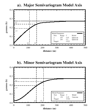
It is often difficult to fit a model semivariogram to both the principle-axis and the minor-axes using traditional methods with anisotropy ratios. Traditionally, models (possibly nested) are modified with anisotropy factors; these represent the relative range of the semivariogram for three orthogonal axes. This technique is restrictive, and this discussion presents a method for relieving this limitation by defining different semivariogram models, independently for each axis. These are referred to as directional semivariograms. The process increases the kriging processing time by 80% to 200%, but the method offers the modeler greater flexibility, and simulation or estimation results that are more representative of the site, because the spatial variation of the data can be more precisely defined.

Introduction

Semivariogram modeling is the foundation for geostatistical analysis, and can also be the most difficult and time consuming portion of the analysis. In part, this is due to the computationally intensive calculations, but it is also due to the difficulty in defining semivariogram models which reasonably honor the experimental semivariograms in the principle and minor search directions. With current techniques that use anisotropy factors (Englund and Sparks, 1988; Journel and Huijbregts, 1978; Deutsch and Journel, 1992), often it is not possible to model all the orthogonal experimental semivariograms exactly. Consequently compromises are required for the definition of one, or even all of the models. If the compromises are not too substantial, then this approach is acceptable, because, generally the kriged results are relatively insensitive to minor changes in the semivariogram. Although this insensitivity offers some comfort, a method that economizes human time and offers more precision is preferable. This paper describes a procedure, which allows the modeler to define a unique semivariogram model for each orthogonal axis of the experimental semivariogram.

Theory

This algorithm uses components of each model to determine (h) values between the axes. Anisotropy factors are not used, rather the modeler specifies the number of nests, sills, ranges, and model structure types independently for each axis. The only requirements are 1) the nugget must be the same for all models, and 2) the total sill must be the same at infinity. These two requirements are not particularly restrictive. Requiring the nugget to be the same is reasonable, because at zero distance, direction is irrelevant. The requirement that the total sill components are equal ensures that the kriging matrix is not singular. If different sills are desired, then this requirement is met by defining an extremely large range for the final nest to make up the balance of the sill component. The error introduced by the final nest has no significant affect on the area of interest.

This technique allows the modeler to honor the results of the experimental semivariogram analysis, thus it is easier to model the data set and the results are more accurate. However, the calculation of (h) is substantially more complex than traditional methods, therefore the method requires computational effort. The additional effort is comparable to the computational effort required for the search procedure and matrix solution portions of the kriging algorithm so, the task, only increased total processing time by about 80% to 200% (based on observed differences in computation time for example data sets). This is acceptable, because the semivariogram model preparation is simplified, and the simulations or estimates more closely honor the spatial statistics of the site.

Two steps of the kriging process are modified to incorporate directional semivariograms into the kriging algorithm: 1) the search for nearest neighbors, and 2) the calculation of the covariance components of the kriging matrix. The first step in estimating the value for a grid location is to find the influential neighboring points. For isotropic situations the nearest sample points are the best estimators. For anisotropic situations, the best estimators are those points with the smallest spatial variance calculated from the model semivariogram ((h)). Using anisotropy factors, the sample point locations are transformed to equivalent isotropic space, using a simple transformation and rotation, based on the orientation of the principle model axis, and the anisotropy factors of the minor-axes. Once transformed, the estimation variance is solely a function of the distance between the grid location and the sample point, therefore (h) doesn't have to be calculated. Conventional techniques (Deutsch and Journel, 1992; Gómez-Hernández and Srivastava, 1990), use Pythagoras' Theorem to find the closest points. When directional semivariogram models are used, direction as well as distance is important. Consequently, a simple transformation and rotation is not possible (Figure 1). For this reason, (h) must be calculated for each sample in the search neighborhood, and those points with the smallest (h) values are the most influential, and thus constitute the most influential neighbors.

FIGURE 1: With directional semivariograms, distance alone does not determine the most influential neighbors. In this example, all points in the minor model axis direction (b) that are separated by less than x₂ (158 m) have smaller

(h)'s than points separated x₁ (109 m) on the major-axis (a). The same is true for x₃ and x₂ respectively.

Once the most influential neighboring data points have been selected, the kriging matrix is solved as usual, with the exception of the (h) calculation. Again, for directional semivariograms, it is not possible to transform points into isotropic space, therefore components of the individual axes must be resolved. Whether (h) is calculated to determine the most influential neighbors or individual components of the kriging matrix, the same technique is used as described in the following section.

Equations and Proof

Calculating (h) to determine the nearest neighbors for a grid location, or to define individual components of the kriging matrix, requires the equation for an ellipsoid:

(1)

Using this equation, it is possible to separate the components of each semivariogram model for any vector (Figure 2). One point is translated to the axis origin, and the second point is positioned at |x|, |y|, and |z|, along the separation vector (h). Here a, b, and c, represent the maximum practical ranges of the semivariogram models along the X-, Y-, and Z-axes respectively. In this section only, when the actual ranges are used, the a_actual, b_actual, and c_actual, subscripts will be used. The practical range refers to the distance where the semivariogram model meets the variance. For the Exponential and Gaussian models, this is defined as 95% of the variance. The practical ranges for different models are defined as (Journel and Huijbregts, 1978):

Model Type	Practical Range
Spherical	range
Exponential	3 x range
Gaussian	sqrt(3) x range
Linear	range

FIGURE 2: Directional semivariogram analysis components.

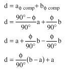
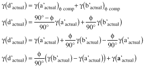
If the unadjusted range and not the practical range is used, the axis defined with the model using the longest practical range will be under-weighted. The equations for determining each component (h)_X,Y,Z and the resultant (h) are derived below. The components of each axis for each structure of the nested semivariogram model can be related through the aspect factors:

(2)

(3)

(4)

Rearranging Equation 1, the ellipsoid factors a², b², and c² for the search vector are solved:

(5)

(6)

(7)

Where a', b', and c' represent the X, Y, and Z-axis intercepts for an ellipsoid passing through an arbitrary point, (x, y, z) along the same vector, where the aspect ratios defined by a, b, and c remain true, the following relationships are also true:

(8a, b, c)

An additional axis, R, is also required. R is defined by the intersection of the X-Y plane, and the vertical plane passing through the point (x, y, z). To determine the semivariogram components, the point r, which lies on the R-axis, vertically below the point (x, y, z) is defined:

(9)

Two additional points of interest are where the semivariogram model ellipsoid and the ellipsoid passing through (x, y, z) cross the R-axis; these are d and d' respectively. Defining these two ellipsoids, with the aspect ratios described above, the components of each semivariogram model can be derived. One new aspect ratio is needed between the R- and Z-axes.

(10)

The distances a, b, c, and d represent the practical model range and a', b', c', and d' represent the practical component range along each axis for the point (x, y, z). The parameter d represents the semivariogram model along the R-axis and is a combination of models a and b. Once a, b, x, and y are known, then d can be determined. For a circle, the angle

is described as:

(11)

Usually, the model semivariogram ellipse (X-Y plane) will not be a circle, therefore the anisotropy must be removed to determine the component angle

. This is the product of y and the aspect ratio of the ellipse (f in the X-Y plane, major/minor dimension):

(12)

The angular components of a and b can then be described by:

(13a, b)

The components can then be summed to calculate d:

(14)

By expanding f and solving, using radians, the equation may be rewritten:

(15)

d' can be determined by proportion:

(16)

Given distances a', b', c', and d', it is possible to solve directly for

(a'),

(b'), and

(c'). To solve for

(d'_actual), the argument used for d is repeated, The components of

(a'_actual) and

(b'_actual) can then be described by:

(17)

(18)

The components are then summed to calculate

(d'_actual):

(19)

By expanding f and solving, the equation may be rewritten:

(20)

To solve for

(e'_actual), where e' is the distance from the origin to the point (x, y, z), steps similar to those used to generate d and

(d'_actual) are required. Allowing

(d'_actual) to be equivalent to

(a'_actual), and

(c'_actual) equivalent to

(b'_actual), this yields:

(21)

These calculation must be evaluated for each nest of the model structure except the nugget (

(h)₀). The nugget, having zero distance, by definition is the same for all axes. This also implies that the number of structures in every direction must be equal. This restriction can be negated by giving undesired nests a zero variance component and the same range as the previous structure. The final

(e'_actual) estimate is the summation on the nugget (i=0) and the nested structure components:

(22)

Positive Definite

The previous equations describe how the orthogonal axes can be independently defined and modeled. A possible problem with this method is it that a number of equations are merged into hybrid equations. In nested structures, this is acceptable, but Myers and Journel (1990) suggest that this may lead to non-invertible covariance matrices (i.e. models that are not positive definite) when the model equations are applied orthogonally. Positive definite matrices are required by the kriging algorithm.

Although we have not proved these hybrid equations yield positive definite matrices, the basic two- and three-dimensional problems described by Myers and Journel, do not occur. Also, several basic tests to validate the assumption of positive definiteness, are not violated (Isaaks and Srivastava, 1989):

i) x^tAx > 0 for all non-zero vectors x.

ii) All the eigenvalues (

_i) of A are greater than 0.

iii) All the upper left submatrices A_k have positive determinants.

iv) All the pivots (d_i, without row exchange) are greater than 0.

This does not prove the equations yield positive definite matrices, but it is a good indicator they do.

Conclusions

This paper describes the calculation method for directional semivariograms. The procedure simplifies modeling the experimental semivariograms, because one need not compromise when selecting model types and sills for each axis. There is an increase in computational effort which increases total processing time (observed times increased 80% to 200%), but this cost is relatively minor when compared to the total time the modeler spends developing semivariogram models. Overall, use of directional semivariogram modeling requires additional computational time, but modeler effort is reduced, and a significant increase in accuracy may be attained.

Acknowledgments

We appreciate the United States Army Corps of Engineers, Waterways Experiment Station for support of this research.

References

Deutsch, C.V. and A.G. Journel, 1992, GSLIB: Geostatistical Software Library and User's Guide. New York, Oxford Press.

Englund, E. and A. Sparks, 1988, GEO-EAS. U.S. Environmental Protection Agency, Environmental Monitoring Systems Laboratory, EPA/600/4-88/033.

Gómez-Hernández, J.J. and R.M. Srivastava, 1990, ``ISIM3D: An ANSI-C Three Dimensional Multiple Indicator Conditional Simulation Program.'' Computers in Geoscience, Vol. 16, No. 4, pp. 395-440.

Isaaks, E.H. and R.M. Srivastava, 1989, An Introduction to Applied Geostatistics. New York, Oxford University Press.

Journel, A.G. and C.J. Huijbregts, 1978, Mining Geostatistics. London, Academic Press.

Myers, D.E, and A. Journel, 1990, Variograms with Zonal Anisotropies and Noninvertable Kriging Systems, Mathematical Geology, Vol. 22, No. 7, pp 779-785.